ACTIVITY 19 - Restoration of Blurred Image

This activity is a demonstration on how to restore an image which is corrupted with a known degradation function such as motion blur and additive noise.

The image degradation and restoration process can be modeled by the diagram shown below.

A degradation function H along with an additive noise terms, n(x,y) operates on an input image f(x,y) producing a degraded image g(x,y). With the given g(x,y) and some knowledge about the degradation function H and additive noise terms n(x,y), we can obtain an estimate restoration f'(x,y) of the original image.

The degraded image is given in the spatial domain

Thus, it can be written in an equivalent frequency domain by getting the Fourier transforms of the corresponding terms.

So we need to have our original image to be transformed in the frequency domain. Now, we will start the degradation of an original image by having our degradation function that will cause the original image to blur. H(u,v) is the Fourier transform of the degradation function given by

where a and b is the total distance for which the image has been displaced in the x- and y- direction, correspondingly and T is the duration of the exposure from the opening and closing of the shutter in the imaging process. We will use a = b = 0.1 and T = 1 and investigate also on other values for these parameters.

The additive noise terms will also be transformed in frequency domain.

To restore these corrupted images, we will apply the Weiner filter expressed by

This expression is also commonly referred to as the minimum mean square error filter or the least square error filter. The terms on the expression are as follows:

This expression is very useful when the power spectrum of the noise and the original image are known. Things can be more simplified when we are dealing with spectral white noise (the power spectrum of the noise is constant). However, the power spectrum of the original image is not often known wherein another approach can be used with the expression

where K is a specified constant. This expression yields the frequency-domain estimate. The restored image must be in the spatial domain which will be obtain by taking the inverse Fourier transform of estimation.

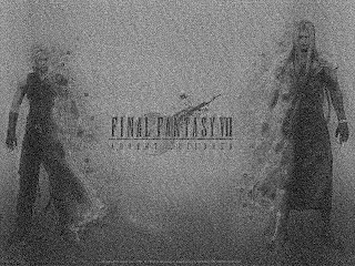
The image utilized for this activity is shown below

**Taken from: http://www.background-wallpapers.com/games-wallpapers/final-fantasy/final-fantasy-vii.html

The following images show the degradation of the original image with the corresponding parameters used. The first set of images has T = 1 and a = b = 0.001, 0.01, and 0.1.

Their corresponding restored images are also obtained and shown below.

We observed that by having small values of a and b, we are putting less blur on the image. Thus, its corresponding Weiner filtered image yields better image.

By keeping a and b constant, T was varied. (T = 0.01, 0.1, 10, and 100 )

Their respective restored image was shown below.

As observed, lesser exposure time makes the noise more obvious with constant values of a and b. On the contrary, greater exposure time will make the blur more visible. The Weiner filter, which works on the blur applied on the original image restores the image with higher exposure time much better.

For cases with unknown power spectrum of the original image, the constant K was varied with a = b = 0.01 and T = 1 . (K = 0.001, 0.01, 0.1 and 1, respectively)

Using a constant value of K shows a significant deviation on the restoration of the degraded image. It shows that knowing the power spectrum of the ungraded image as well as the power spectrum of the added noise is crucial in filtering blurred images. However, in instances that the two parameters are unknown, choosing a good value of K will yield a more enhanced image.

I will grade myself 9/10 for this activity. I was able to understand the activity and obtain the needed output given a short working time. However, I know that there are still so much to learn from this activity. I acknowledged Gilbert for helping me finish this activity.

The code below was use in implementing the Weiner filter on the degraded images.

image = gray_imread('FF7.bmp');
noise = grand(size(image,1), size(image,2), 'nor', 0.02, 0.02);

a = 0.01;
b = 0.01;
T = 1;

H = [];
for i = 1:size(image,1)
for j = 1:size(image,2)
H(i, j) = (T/(%pi*(i*a + j*b)))*(sin(%pi*(i*a + j*b)))*exp(-%i*%pi*(i*a + j*b));
end
end
F = fft2(image);
N = fft2(noise);

G = H.*F + N;
noisyblurredimage = abs(ifft(G));

scf(1);
imshow(noisyblurredimage, []);
imwrite(normal(noisyblurredimage), 'filename.bmp');

// Weiner filtering

Sn = N.*conj(N);
Sf = F.*conj(F);
K = Sn./Sf;
W = H.*conj(H);

Fres = ((1)./H).*((W)./(W+K)).*G;
Fres = abs(ifft(Fres));
scf(2);
imshow(Fres, []);
imwrite(normal(Fres), 'filename.bmp');

ACTIVITY 18 - Noise Models and Basic Image Restoration

This activity aims to be able to be familiar with different noise models by applying them on an image and then restore the degraded image by implementing various spatial filters.

Noise are random variables that are characterized by a probability density function or PDF. In this activity, different noise models were applied on an ungraded image.

First is the Gaussian noise which is also known as normal noise model. The PDF of a Gaussian random variable, z, is given by
where z represents gray level, myu is the average value of z and sigma is its standard deviation.

Next is the Erlang or Gamma noise which is given by
The mean and variance of this density are given by
, respectively.

The Exponential noise has the PDF given by
and has the mean and variance given by
Then we have the Uniform noise with PDF given by
and has mean and variance given by
The Impulse or Salt-and-Pepper noise has PDF given by
Finally, we have the Rayleigh noise which has the PDF given by
The mean and variance of the Rayleigh noise is given by
These noises were created using the built-in function grand in Scilab and then applied on an ungraded image.

The corrupted images were then restored using different filters. First is the Arithmetic mean filter. represent the set of coordinates in a rectangular subimage window of size m x n, which has center at point (x,y). The arithmetic mean filtering process computes the average value of the corrupted image g(x,y) in the are defined by S sub xy. The value of the restored image f at point (x,y) is simply the mean computed using the pixels int he region defined by S sub xy.


The Geometric mean filter will restore an image with the use of the equation below.
The Harmonic mean filtering operations is given by the expression
This filter works better for salt noise than the pepper noise.

The Contraharmonic mean filtering operations yields a restored image based on the expression
where Q is the order of the filter. This filter is suited in treating salt-and-pepper noise. Positive values of Q will eliminate pepper noise while negative values omits salt noise. Thus, it cannot remove both noise simultaneously.


I was able to finish this activity and obtained MANY images. All files were deleted after the CSRC reset our computers. Unfortunately, I didn't have backup of my files. I guess, 5/10 is enough for me since I don't have pictures to show that I have finished this activity. :-(
Anyway, I want to thank Gilbert for guiding me in this activity.

ACTIVITY 17 - Photometric Stereo

In this activity, we estimated and then extracted the shape of an object from shadow with the use of different sources and shading models.

First, we utilized the images of of synthetic spherical surfaces that are illuminated by a far away point source.

It looks like there are no significant difference among the pictures above but the shading of the images tells much information about the surface of the object. It gives the intensity captured by the camera at point (x,y). These images are captured from the surface of the object with the sources located respectively at
This numbers were put into matrix form where each row is a source and each column is the x,y, and z component of the source.
Now we are given with I and V which is related by
We can solve for the surface normal vector by first getting g with the use of the equation
This is the reflectance of the of the object at the point normal to the surface. The surface normal vector is obtained from g divided by its magnitude
From the surface normals, we computed the elevation z = f(u,v) and the 3D plot of the shape of the object was displayed.

The surface normals (nx, ny, nz) obtained using photometric stereo are related to the partial derivative of f(x,y) as
Then, the surface elevation z at point (u,v) which is given by f(u,v) is evaluated by a line integral
Finally, the 3D plot of the shape of the object was displayed.
The shape of the object with spherical surfaces was successfully extracted and displayed.

The Scilab code used in this activity was shown below. I want to acknowledge the help of Gilbert in working on this activity.

loadmatfile('Photos.mat');

// intensity captured by camera at point (x,y)
I1 = matrix(I1, 1, size(I1, 1)*size(I1, 2));
I2 = matrix(I2, 1, size(I2, 1)*size(I2, 2));
I3 = matrix(I3, 1, size(I3, 1)*size(I3, 2));
I4 = matrix(I4, 1, size(I4, 1)*size(I4, 2));
I = [I1; I2; I3; I4];

// location of the point sources
V1 = [0.085832, 0.17365, 0.98106];
V2 = [0.085832, -0.17365, 0.98106];
V3 = [0.17365, 0, 0.98481];
V4 = [0.16318, -0.34202, 0.92542];
V = [V1; V2; V3; V4];

// calculation of surface normal vector
g = inv(V'*V)*V'*I;
magnitude = sqrt((g(1,:).^2) + (g(2,:).^2) + (g(3,:).^2))+.0001;
n = [];
for i = 1:3
n(i,:) = g(i,:)./magnitude;
end

// computation for the elevation z = f(x,y)
nx = n(1,:);
ny = n(2,:);
nz = n(3,:) + 0.0001;
dfx = -nx./nz;
dfy = -ny./nz;
z1 = matrix(dfx,128,128);
z2 = matrix(dfy,128,128);
Z1 = cumsum(z1,2); // integration from 0 to u
Z2 = cumsum(z2,1); // integration from 0 to v
z = Z1 + Z2;
scf(0);
plot3d(1:128, 1:128, z);

ACTIVITY 16 - Neural Networks

This activity is again related from the two previous activities, Activity 14 and 15. The purpose of this activity is to classify objects from their corresponding class using neural networks. The features of of the samples from the two classes used in Activity 15 was also used in this activity. The Clorets mint candy was tagged with the value of 0 while the Pillows chocolate snack was tagged with the value of 1.

The code below was made to implement the Artificial Neural Network algorithm.

clorets_train = fscanfMat('clorets_train.txt');
pillows_train = fscanfMat('pillows_train.txt');
clorets_test = fscanfMat('clorets_test.txt');
pillows_test = fscanfMat('pillows_test.txt');

cp_train = [clorets_train; pillows_train];
cp_train(:,1) = cp_train(:,1)/max(cp_train(:,1));
cp_train = cp_train';
cp_test = [clorets_test; pillows_test];
cp_test(:,1) = cp_test(:,1)/max(cp_test(:,1));
cp_test = cp_test';

rand('seed', 0);

network = [4, 4, 1];
groupings = [0 0 0 0 0 1 1 1 1 1];
learning_rate = [1, 0];
training_cycle = 1000;

training_weight = ann_FF_init(network);
weight = ann_FF_Std_online(cp_train, groupings, network, training_weight, learning_rate, training_cycle);
class = ann_FF_run(cp_test, network, weight);

** the source code was from Cole Fabro's work

The training parameters, learning rate and training cycle were tuned. It was observe that for a given training cycle, the recognition is more accurate with large learning rate. On the other hand, with the learning rate being constant, the recognition is also more accurate.

I will give myself a grade of 10/10 for this activity. Although the code was already given, I fully understand the effect of tuning the training parameters on the accuracy of the recognition. I thank Gilbert for helping me on this activity.