This activity was done to be able to qualify different objects through their various characteristics such as shape, size and color by pattern recognition. A set of features of the objects will be used as pattern. We aim to identify from where class an unknown object belongs.
First, three sets of objects were assembled. Each set represent a class composing of 10 samples. This activity utilized
Clorets mint candy,
Pillows chocolate snack and
Potchi gummy candy. The picture of the objects obtained was shown below.

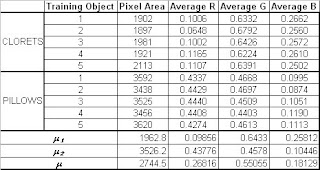
Each of the three class was divided into two sets. The first five samples will be the training set while the remaining five will serve as the test set. The pixel area, the average normalized chromaticity values in red, green and blue will be used as features for pattern recognition. These features were obtained using the techniques that have been learned in previous activities. The pixel area was determined by thresholding, inverting and counting the number of pixels of the black and white image of the set objects. On the other hand, the chromaticity values were obtained by using the non-parametric segmentation technique. After obtaining each feature, they are arranged into matrix form producing the feature vector. The training feature vectors were separated from the test feature vectors. From the training feature vectors, the mean feature vector was determined from the expression

Here,
N is the total number of samples in the class
wj and
xj is feature vector in the training set of the corresponding class. Basically, this is just the mean of the pixel area and the normalized chromaticity values for red, green and blue from 5 samples comprising the training set. Each sample from the test set will be compared to the mean feature vector, which is a 1 x 4 matrix. This will be done through minimum distance classification where the Euclidean distance is applicable given by

where x is the feature vector of the test set and j is the number of classes which in this case is 3.
The feature vector of every sample on each set and their corresponding mean feature vector is shown in the table below.

The resulting mean distance and the classification of the samples from the test set was shown in another table below.

As have been observed, the calculated mean distance,
D is relatively larger when the test sample does not belong to the class. Relatively small mean distance tells that the test sample belongs to the class. However, there is a deviation between the
Clorets and
Potchi sample. Some
Clorets test samples were classified as
Potchi while some
Potchi samples were classified as
Clorets. We can say that the deviation was brought by the shape of both sample. Overall, the technique was useful in classifying objects of different characteristics.
I will give myself a grade of 10/10 in this activity. I was able to understand how to use the characteristics of objects as pattern in classifying them through pattern recognition. I had a hard time capturing pictures of the samples that can be threshold correctly in order to use the
bwlabel function of
Scilab in getting the pixel area. After obtaining the picture, acquiring the data was made easy with the help of Gilbert.
The code below was utilized in this activity.
image1 = 1-gray_imread('bwclorets1.bmp');
// Area computation for training set
[L, n] = bwlabel(image1);
area = [];
for i = 1:n
area(i) = sum(i==L);
end
mean_area = mean(area(1:5));
for i=1:10
image =imread('clorets'+string(i)+'.bmp');
patch = imread('patchclorets.bmp');
r = image(:,:,1);
g = image(:,:,2);
b = image(:,:,3);
rp = patch(:,:,1);
gp = patch(:,:,2);
bp = patch(:,:,3);
R = r./(r+g+b);
G = g./(r+g+b);
B = b./(r+g+b);
Rp = rp./(rp+gp+bp);
Gp = gp./(rp+gp+bp);
Bp = bp./(rp+gp+bp);
Rmu = mean(Rp);
Gmu = mean(Gp);
Rsigma = stdev(Rp);
Gsigma = stdev(Gp);
// Non-parametric Segmentation
BINS = 256;
rint = round( Rp*(BINS-1) + 1);
gint = round (Gp*(BINS-1) + 1);
colors = gint(:) + (rint(:)-1)*BINS;
hist = zeros(BINS,BINS);
for row = 1:BINS
for col = 1:(BINS-row+1)
hist(row,col) = length( find(colors==( ((col + (row-1)*BINS)))));
end;
end;
rib = R*255;
gib = G*255;
[a, b] = size(image);
np = zeros(a, b);
for r = 1:a
for s = 1:b
c = round(rib(r, s)) + 1;
d = round(gib(r, s)) + 1;
np(r,s) = hist(c, d);
end
end
// Mean color per channel
imageR = [];
imageG = [];
imageB = [];
[x , y] = find(np ~= 0);
for j=1:length(y)
imageR = [imageR, R(x(j),y(j))];
imageG = [imageG, G(x(j),y(j))];
imageB = [imageB, B(x(j),y(j))];
end
mean_imageR(i,:) = mean(imageR);
mean_imageG(i,:) = mean(imageG);
mean_imageB(i,:) = mean(imageB);
end
mean_imageR_training = mean(mean_imageR(1:5));
mean_imageG_training = mean(mean_imageG(1:5));
mean_imageB_training = mean(mean_imageB(1:5));
M=[mean_area,mean_imageR_training,mean_imageG_training,mean_imageB_training];
// Area computation for test set
image2 = 1-gray_imread('bwclorets2.bmp');
[L, m] = bwlabel(image2);
area2 = [];
for i = 1:m
area2(i) = sum(i==L);
end
// Mean Distance
D = [];
X = [];
for i=6:10
X=[area(i-5),mean_imageR(i),mean_imageG(i),mean_imageB(i)];
d = X-M;
D = [D, sqrt(d*d')];
end
 It looks like there are no significant difference among the pictures above but the shading of the images tells much information about the surface of the object. It gives the intensity captured by the camera at point (x,y). These images are captured from the surface of the object with the sources located respectively at
 This numbers were put into matrix form where each row is a source and each column is the x,y, and z component of the source.
 Now we are given with I and V which is related by
 We can solve for the surface normal vector by first getting g with the use of the equation
 This is the reflectance of the of the object at the point normal to the surface. The surface normal vector is obtained from g divided by its magnitude
 From the surface normals, we computed the elevation z = f(u,v) and the 3D plot of the shape of the object was displayed.
 Then, the surface elevation z at point (u,v) which is given by f(u,v) is evaluated by a line integral
 Finally, the 3D plot of the shape of the object was displayed.
 The shape of the object with spherical surfaces was successfully extracted and displayed.


