ACTIVITY 4 - Enhancement by Histogram Manipulation

In this activity, grayscale images will be enhanced by manipulating their histogram which is the graylevel probabilit function or PDF when normalized. Histogram can be modified by having the cumulative distribution function (CDF) of the image and a desired CDF. The image was modified by backprojecting the grayscale values of the desired CDF.

A grayscale image with poor contrast was downloaded from the internet. Then the grayscale histogram of the image was obtained using Scilab.

grays = gray_ imread('gray_image.jpg'); //read from grayscale file

//compute and plot the histogram
j=1;
pix = [];
for i = 0:255
[x,y]=find(grays==i);
pix(j)=length(x);
j=j+1;
end





















The grayscale image was show above along with its grayscale histogram. We then determine the CDF of the image from its PDF. The CDF is given by
where p1(r) is the PDF of the image. The CDF of the grayscale image above was shown at the left side below.

We are going to remap the grayscales of the image in a way that the resulting CDF of the reconstructed image will look like our desired CDF. The CDF of a uniform distribution is a straight increasing line. If we wanted our image to have a uniform distribution of gray values, we will use a straight line, shown above right as our desired CDF.


The process of backprojection was illustrated below.


Each pixel value has a CDF value. This value was traced in the desired CDF. The pixel value will then be replaced by the new pixel value in the desired CDF.

b = pix;
c = cumsum(b);
f = c/max(c);
x = 0:255;

imsize = size(grays);
dCDF = x;

for i = 1:imsize(1)
for j = 1:imsize(2)
ind= find(x == grays(i, j));
grays(i, j) = f(index);

The resulting image was shown below.
The transformed image shows a significant increase in contrast. This image is now called a histogram equalized image.To have more idea about the image, we displayed its grayscale histogram and its CDF.
















Compared with the original histogram, the histogram of the transformed image showed a more uniform distribution of grayvalues. As with our goal, the CDF of transformed image looked like just the same as the desired CDF.
----------------------------------------------------------------------------------------------------------------
We have manipulated the histogram of a grayscale image with the use of a linear desired CDF. However, the human eye has a nonlinear reponse. So we can mimic the human eye response by using a nonlinear CDF. We can use a tanh function as our desired CDF which is nonlinear. Its plot was shown below.

x = 0:255;
tanhf = tanh(16.*(x-128)./255);
tanhf = (tanhf - min(tanh))./2;

Again, the backprojection was done. The CDF value of the pixel value was traced along the CDF value of the desired CDF. The pixel value in the desired CDF will be the new pixel value.

b = pix;
c = cumsum(b);
f = c/max(c);
x = 0:255;

imsize = size(grays);

for i = 1:imsize(1)
for j = 1:imsize(2)
ind = find(x == grays(i, j));
pixel1 = f(index);
pixel2 = find(tanhf<= pixel1); grays(i, j) = (pixel2(max(pixel2)));

The transformed image using a non-linear CDF was shown below.
Clearly, the transformed image is not as good as the image transformed using linear CDF. The image becomes darker with very poor contrast. We display its grayscale histogram and its CDF.















We can see from the grayscale histogram the distribution of gray values at a certain region at the center. The CDF shows that we were able to transformed the grayscale image base from the desired CDF. However, we were not able to enhance the contrast of the gray image.

I give myself a grade of 9 for this activity. I was able to easily understand the backprojection of pixels however, I had a hard time implementing it in a code. Also, I was able to show the effect of having a linear and non-linear CDF desirable for transforming a grayscale image. In this activity, I learned how to qualify an image with just looking on its grayscale histogram. The more uniform the distribution of the grayscale values, the better the contrast of the grayscale image. I acknowledged the help of Gilbert, who tirelessly helped me debug my code and waited for me until I gathered all my results.

ACTIVITY 12 - Color Image Segmentation

In this activity, we are going to pick out a region of interest from the rest of the image through image segmentation.

A digital image of 3D objects, shown below, was utilized in this activity. Different brightly colored candies are shown in the image.

We cropped a monochromatic region of interest in the scene. In this case, we wanted the blue candies to be our region of interest.

We notice that these objects found in the image, as well as the cropped image have shading variations which is inherent in 3D objects. To separate brightness and chromaticity (pure color) information, it is better to represent the color space by the normalized chromaticity coordinates or NCC. The normalized chromaticity coordinates can be obtained by dividing each pixel from each channel by the summation of the pixel corresponding on each channel.

This was implemented by the code below.

image =imread('candy.jpg');

patch = imread('patch.jpg');

r = image(:,:,1);

g = image(:,:,2);

b = image(:,:,3);

rp = patch(:,:,1);

gp = patch(:,:,2);

bp = patch(:,:,3);

R = r./(r+g+b);

G = g./(r+g+b);

B = b./(r+g+b);

Rp = rp./(rp+gp+bp);

Gp = gp./(rp+gp+bp);

Bp = bp./(rp+gp+bp);

Parametric Segmentation

The Gaussian PDF in the r values was derived using the equation

where sigma is the standard deviation and mu is the average of the normalized chromaticity coordinate in red of the patch image. The same equation was used for g values.

Rmu = mean(Rp);

Gmu = mean(Gp);

Rsigma = stdev(Rp);

Gsigma = stdev(Gp);

pr = (1/(Rsigma*sqrt(2*%pi)))*exp(-((r-Rmu).^2)/(2*(Rsigma)^2));

pg = (1/(Gsigma*sqrt(2*%pi)))*exp(-((g-Gmu).^2)/(2*(Gsigma)^2));

Then, the joint probability was taken as the product of rho(r) and rho(g).

product = round(pr.*pg);

The resulting image was shown below.

Non-Parametric Segmentation

The 2D histogram of the ROI was obtained using the give code below.

BINS = 256;

rint = round( Rp*(BINS-1) + 1);

gint = round (Gp*(BINS-1) + 1);

colors = gint(:) + (rint(:)-1)*BINS;

hist = zeros(BINS,BINS);

for row = 1:BINS

for col = 1:(BINS-row+1)

hist(row,col) = length( find(colors==( ((col + (row-1)*BINS)))));

end;

end;

scf(1);

mesh(hist);

To test the correctness of the histogram, we compare the location of the peaks with the rg chromaticity diagram (at the right). Clearly, we can see that the histogram of the ROI peaks at the are corresponds to the blue color in the rg chromaticity diagram. This histogram willl be important in segmenting the image using histogram bakcprojection.

This histogram backprojection is similar to what has done in Activity 4 excepth that in this case, the histogram is in 2D. Backprojection was done by replacing the value of the pixel location by its histogram value in chromaticity space. This was implemented by the code below.

rib = R*255;

gib = G*255;

[a, b] = size(image);

np = zeros(a, b);

for i = 1:a

for j = 1:b

c = round(rib(i, j)) + 1;

d = round(gib(i, j)) + 1;

np(i, j) = hist(c, d);

end

end

scf(2);

imshow(np);

The resulting image was shown below.

By implementing two different segmentation techniques, different parts of the region of interest was segmented. Parametric segmentation enables us to segment the outer part of the blue candies while non-parametric segmentation enables us to segment the inner body of the blue candies. The non-parametric segmentation favors in segmenting the region of interest although not all ROI were segmented.

I give myself a grade of 10 for finishing this activity. I was able to implement the parametric and non-parametric segmentation on an image composed of an ensemble of colored objects.

I would not have finished my blogs without the overwhelming help of Gilbert and Rommel. Gilbert was the one who patiently discussed every activity with me. He help me a lot in understanding previous activities. Rommel, after finishing his blog was able to lend me his laptop. It was a big help considering that I did not work on my blog in a computer shop for almost 4 hours.

:-) I acknowledged all my classmates who made me feel their concerns for me. I want to extend my deepest gratitude for all of you guys.

ACTIVITY 11 - Color Image Processing

Primarily, the objective of this activity is to be able to enhanced an image that is wrongly white-balanced. Images of an ensemble of colorful objects were captured using a digital camera with different white balance settings.

White Balancing Setting: Fire

White Balancing Setting: Shade

White Balancing Setting: Fluorescent-1

White Balancing Setting: Fluorescent-2

White Balancing Setting: Fluorescent-3

White Balancing Setting: Incandescent

Different white balancing settings resulted to different qualities of images. The Fire and Shade are almost the same resulting to a slightly darker image than what was taken. Fluorescent-1 settings resulted to a brownish image. Fluorescent-2 and Fluorescent-3 produced shades of blue images. The Incandescent setting produced a more bluish image. Obviously, this image is wrongly balanced.

White Patch Algorithm

Using the image captured by the camera in Incandescent setting, the White Patch algorithm was implemented. First, a patch of an white object in real world which appears differently in the image was cropped.
The RGB values of pixels belonging to this white object: Rw, Gw, and Bw was taken. And then, all pixels in the red layer, green layer and blue layer of the image was divided by their corresponding Rw, Gw and Bw. This was implemented with the code below.

image = imread('filename.jpg');
w = imread('wpatch.jpg');

rw = sum(w(:,:,1))/length(w(:,:,1));
gw = sum(w(:,:,2))/length(w(:,:,2));
bw = sum(w(:,:,3))/length(w(:,:,3));

nr = image(:,:,1)/rw;
ng = image(:,:,2)/gw;
nb = image(:,:,3)/bw;

The resulting image was then displayed as shown below.

Compared with the wrongly white balanced image, the resulting image is less brighter as the bluish color decreases. White hues that appear bluish in the wrongly balanced image now appear more white. The White Patch algorithm assumes that the maximum response of the image is caused by the white patch. Thus, by dividing each channels of the image with the constants determined from the white patch we are essentially bringing back true colors of the image.

Gray World Algorithm

The Gray World algorithm was also implemented on the image captured using Incandescent setting. For this algorithm, the R, G and B layers of the unbalanced image were averaged and let to be Rw, Gw, and Bw, respectively. Then the original R, G and B layer values were divided by their corresponding constant.

image = imread('filename.jpg');

rw = sum(image(:,:,1))/length(image(:,:,1));
gw = sum(image(:,:,2))/length(image(:,:,2));
bw = sum(image(:,:,3))/length(image(:,:,3));

nr = image(:,:,1)/rw;
ng = image(:,:,2)/gw;
nb = image(:,:,3)/bw;

The resulting image was displayed below.
The image looks old after the implementation of Gray World algorithm. The blue hues also lessen and the white hues look grayish. The Gray World algorithm assumes that the average of the colors on each channels of the image taken in normal light is gray. Using the Incandescent setting in capturing the image, we have disrupted the Gray World assumptions. We force the Gray World assumption again by dividing each channel by their average. Thus, we are reaquiring the true color of the image in real world.

Doing both algorithm with the other images will result to the same image as shown above for white patch and gray world algorithm. Implementing both algorithms is reacquiring the true colors of the image based on certain assumptions. However, it turns out that the White Patch is better than the Gray World algorithm.
------------------------------------------------------------------------------------------------------------

In this part of the activity, the white patch and gray world algorithm were implemented on an image of objects with the same hue (in this case, green).
The image above was obviously wrongly white balanced. After implementing the two algorithm as in above procedure, the resulting images were shown below.

White Patch Algorithm

Gray World Algorithm

The white patch algorithm uses the white wall at the background of the image. Clearly, the original color was reacquired using white patch algorithm. Gray world algorithm allows the removal of the bluish hue in the image. However, the image becomes slightly reddish. This is because the unbalanced image mainly composed of green hues.

For this activity, I will get 10/10. By producing images from each algorithm, I was able to understand how the white patch and gray world algorithm assumes the color of the real world. Applying these algorithm on an image captured with colored lighting (i.e. Incandescent white balancing setting ) will reacquire the true colors of the image. However, after finishing the activity, it turns out that for the images used, the White Patch algorithm assumes a better color of the real world. I acknowledged Gilbert for discussing the activity with my and for lending me pictures he captured.

ACTIVITY 10 - Processing Text

This activity aims to extract handwritten text from an imaged document with lines. In order for the handwriting to be recognized, individual letters must be extracted. We will again use all the image processing techniques we have learned.

The image below will be utilized for this activity.

A portion of the image was cropped with handwritten text together with lines in the form.

We can see from the horizontal lines that the image is tilted. With the use of mogrify function which is built-in function is Scilab, the image was rotated. The image below shows the rotated image.

Now that we have rotated the image, we will have to remove the horizontal lines from the form using image processing techniques. First we have to display the FT of the image in logarithmic form. In doing this we will have the idea where the frequencies of the horizontal lines lie, just like in the previous activities. We will design the filtering mask by blocking the frequencies the correspond to the unwanted horizontal pattern.

The image at the left is the FT of the image in logarithmic form and the image at the right shows the filtering image. We can see on the filter how we are able to block the frequencies of the horizontal line. The resulting image is shown below.
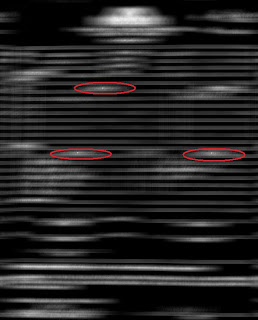
This image resulted from the filtering technique applied to the cropped portion of the original image. After the removal of the horizontal lines, the image was then inverted. We notice that the background becomes black and the texts become white. This was done in able for us to use the morphological operations we have learned. We recall that these operations applies only to the "white" portion of the image which is our object.

But before implementing morphological operation, we have to binarize the image first. We look for the best threshold such that the object is well separated with the background. And then, the dilate and erode functions were used. The combination of the two operations were done until the best extraction of the texts was produced.
The image above shows the final extraction of the text image. From this image, we can see the significant separation of each text in the word "remote control". The rest of the words, although the letters are being separated from each other somehow, are still unrecognizable. From the beginning, we have a very poor image. We can compare the separation of the letters by counting the number of blobs produced using the bwlabel function. Supposedly, there are 46 letters in the cropped portion of the image. The number of blobs produced after doing image processing techniques was found to be 31. Thus, the image processing techniques applied to the image has a significant effects on the separation of each text.
-------------------------------------------------------------------------------------------------
In this part, we will use the template matching technique we have learned in Activity 6.C to find the instances of the word "DESCRIPTION" in the whole image.

First, we binarize the whole image and find the best threshold. Then we cropped the word DESCRIPTION from the image and pasted it on a black background with the same size as the image which will be our template.




















And then the correlation technique was applied. The FT of the template was multiplied with the conjugate of the FT of the image. Then the fftshift of the product was taken.
The image above shows three instances of the word DESCRIPTION in the image which is what we have expected. We can see these instances from the bright spots where the correlation is high.

I want to give myself a grade of 9 in this activity. Although I have used the image processing techniques I have learned, I was not able to come up with a more enhanced text image. Again, Gilbert was acknowledged for this activity.

ACTIVITY 9 - Binary Operations

This activity is an integration of everything we have learned to determine the best estimate area in pixel count of simulated "cells". In addition, we are going to use more morphological operators such as the closing and opening operator for enhancing and analyzing binarized images.

The image above which is an image of scattered punched paper digitized using a flatbed scanner was utilized in this activity. We imagine that the circles are imaged cells on a slide. Our primary goal: estimate the area of ONE "cell".

We begin the task by dividing the whole image into 256 x 256 subimages. Each subimage was opened in grayscale. A sample subimage was shown below.
The threshold of the subimage was obtained from its histogram. The threshold is important in order to separate the background from the cell, which is our region of interest (ROI). Then the subimage was binarize using the Scilab function im2bw.
In order to emphasize the separation of ROI from the background, we implemented opening and closing operator using the dilate and erode functions which are built-in functions in Scilab.

//opening
image1 = erode(dilate(image));
Opening operator removes small objects inside the cell.

//closing
image2 = dilate(erode(image1));
While closing operator removes small holes on the background.

After doing morphological operations, we have now a cleaner image of the cells. Then, contiguous blobs are formed within each subimage. The bwlabel function was used to label each blob on the subimage. The area or the number of pixels of each blob was measured from each subimage and then tallied.

//area computation
[L, n] = bwlabel(image2);
area = [];
for i = 1:n
area(i) = sum(i==L);
end
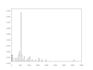
From the histogram of the areas, the average of the area was taken from the range of areas with high occurrences. The calculated mean area was found to be 526 pixels with a standard deviation of 24.67. In order to verify this calculation, a single "cell" was taken from the whole image, binarized and then summed in order to get the area in pixel.
The area of a single cell was measured to be 535 pixels. In comparison to the calculated area, a 1.76% error was obtained.

I will give myself a grade of 10/10 for finishing this activity. Aside from obtaining a small percentage error, I understand most part of the activity. I was able to apply image processing and area calculation techniques I have learned in previous activity. I think that using bwlabel function in calculating the area of each blob in a subimage was a clever idea. As always, I want to acknowledged Gilbert in helping me understand the activity.