ACTIVITY 2 - Area Estimation of Images with Defined Edges

In this activity, our goal is to be able to compute for the area of images with the use of Green's Theorem. First, we created images (with black background and white as the object) using MS Paint.

Then, the areas of the object on each image were calculated using Green's equation given by
I create a code using scilab that computes for the area of the object in a black and white image. This code utilizes Green's equation. The computed area was then compared to the area obtained by summing up all 1's in the image (white object).

SOURCE CODE:

image = imread('tri 4900.JPG');//read image from file
bin = im2bw(image, 0.5);//convert image to black and white
[x,y] = follow(bin);//follow the contour of the object
plot2d(x,y);//plot of the contour

//Green's Theorem
area=[];
for i = 1:(length(y)-1)
area(i) = x(i)*y(i+1)-y(i)*x(i+1);
end
areatot =((sum(area))/2)

//pixel area
pixarea = sum(bin)-length(y)

//percentage error
%err = abs((areatot-pixarea)/pixarea)*100

By using the syntax 'follow', Greens's equation disregards the contour in computing for the area. In order to compensate the pixel area, we have to subtract the perimeter of the contour in the sum of the pixel area. The table below shows the computed areas and corresponding percent error. I give myself a 10/10 in this activity. I understand well the objective of the activity and thus being able to create a code. I acknowledged Raffy and Gilbert for agreeing with me about the fact that 'follow' disregard the number of pixels of the contour using Green's equation.

ACTIVITY 3 - Images Types and Basic Image Enhancement

In this activity, we collected digitized images from the web and classified them into four types: binary images, grayscale images, indexed images and truecolor images. Using the imfinfo of Scilab-4.1.2, the properties of each image were determined.

BINARY IMAGE

FileSize: 344
Format: PNG
Width: 248
Height: 248
Depth: 8
StorageType: indexed
NumberOfColors: 2
ResolutionUnit: centimeter
XResolution: 72.000000
yResolution: 72.000000

***http://www.true-binary.com/true-binary.png

GRAYSCALE IMAGE

FileSize: 28244
Format: PNG
Width: 290
Height: 300
Depth: 8
StorageType: indexed
NumberOfColors: 256
ResolutionUnit: centimeter
XResolution: 14.960000
YResolution: 14.960000

***http://peps.redprince.net/peps/tiger-Q300.png

INDEXED IMAGE

FileSize: 6989
Format: GIF
Width: 491
Height: 334
Depth: 8
StorageType: indexed
NumberOfColors: 4
ResolutionUnit: centimeter
XResolution: 72.000000
YResolution: 72.000000

**http://www.springboardmagazine.com/SpringImage s/tiger.gif

TRUE COLOR IMAGE

FileSize: 31029
Format: JPEG
Width: 625
Height: 450

Depth: 8
StorageType: truecolor
NumberOfColors: 0
ResolutionUnit: centimeter
XResolution: 100.000000
YResolution: 100.000000

***http://animal.discovery.com/mammals/tiger/pictures/tiger-picture.jpg

----------------------------------------------------------------------------------------------------

I looked for a 3 1/2 diskette and had it scanned. Then I got its properties using imfinfo.
The image was then converted into grayscale. I created a code that will compute and plot the histogram of the scanned image. It is clearly shown from the histogram that the region of interest (ROI) is well separated from the background which is expected.With the use of im2bw, the image was converted into black and white using the best threshold (for this case, 0.5). For a nicer image, I used MS Paint. To get the area of the image, I applied the area calculation program I made for Activity 2. With this procedure, I got a 0.33 % error from the area calculated.

I will give myself a grade of 9/10 for this activity. I finished this activity late because I had a hard time looking for an object to be scanned. I thought that any little object I could think of might have already done by my classmates. I acknowledged again the help of Gilbert and Raffy for answering all questions I had in mind.

ACTIVITY 1 - Digital Scanning

Primarily, this activity aims to find the numerical values of a digitally scanned hand-drawn plot with the use of ratio and proportion.

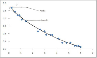
First, I looked for a hand-drawn graph from an old journal and I found this plot from Annals of Chemistry, 1940.

This graph relates the carbon dioxide output from washed potato tubers under aerobic and anaerobic conditions.

I started noting down the pixel values of each data point by first having a conversion factor which relates the number of pixels to a certain number of physical value along both x and y axis.

For the x-axis, the ratio is 222:1 pixels and for the y-axis, there is 1440:1 pixels ratio. With these ratios in hand, I was able to tabulate the number of pixels of each data points and their equivalent physical values on each axis.

Finally, a reconstruction of the graph was done in OpenOffice.org Calc.

The plot above shows a decent reconstruction of the original graph. With the original graph being placed at the background of the reconstructed graph, we can see the correspondence among each data points with insignificant deviations. The trendline imposed on the reconstructed graph also fits the trendline of the original graph.

I evaluate myself with a grade of 10/10 from being able to find the numerical values of a hand-written graph by utilizing the ratio of number of pixels to number of physical value. I exerted enough effort to finish this activity on time. I also acknowledge the help of Raffy, Gilbert and Kaye in discussing the way on how to begin with the activity.